Meta-Analysis Tool

The Metapsy meta-analysis tool has been developed to make the available datasets more accessible for various stakeholders, without requiring programming skills. These graphical user interfaces allow to analyze existing versions of datasets using state-of-the-art meta-analytic methods. An overview of available tools is provided on the Metapsy website.
Starting Page
The starting page of each meta-analysis tool displays some basic information on the available dataset. To the right, the number of available studies and the dataset version is shown.

The additional information section at the bottom contains further links and information on the dataset. It also provides the link to the R script that was used to simplify the data for the online meta-analysis tool. Most datasets are simplified slightly to reduce the complexity of analyses within the app. A main step conducted in all simplification scripts is to aggregate all effect sizes within studies. This is done using the runMetaAnalysis function in metapsyTools, which by default assumes a constant sampling correlation of $\rho$ = 0.6 (i.e., it is assumed that multiple effect sizes collected in the same study are correlated by r = 0.6).
The aggregation is conducted on an arm level. This ensures that multiple treatment arms within the same trial are preserved in the provided data, and that differences can be analyzed in separate subgroup analyses. Please note that this approach may not fully remove effect size dependencies when there are multi-arm trials in the data (e.g., trials that compare two psychological treatments to the same control group). It may be advisable to conduct further sensitivity analyses (e.g. using metapsyTools) if a strict control for potential unit-of-analysis errors is desired.
In the footer, the starting page also provides a link to the documentation entry of the database; as well as a contact address in case the application does not function as intended.
The green “circle arrow” button in the top-right can be used to re-load the application. Please note that this removes previous results obtained using the tool. The reload button is available on all pages of the application.
Data Selection
The data selection pane can be opened by clicking the “Starting Analyzing” button. This page shows a table of the provided data, along with the calculated effect sizes (expressed as Hedges' g) and their estimated sampling variances.
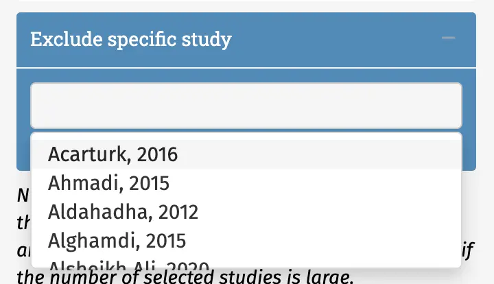
The right sidebar provides a selection of buttons and sliders that can be used to filter the database as needed. To open a filter, one has to click the “+” sign to the right of each provided variable. The blue box at the end of the sidebar can be used to exclude specific studies within the database.
Once the desired filters have been selected, the Update Table button must be clicked to filter the database. The displayed table is then re-rendered and will only contain the studies fulfilling the selected criteria. A line at the very end of the table can be helpful to see how many effect sizes can be pooled using the current filters.
Before running the meta-analysis, please make sure to always click on “Update Table” first. Otherwise, your selected filtering criteria will not be implemented by the application.
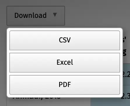
The “Download” button in the top-left corner of the table can be used to download the selected dataset as a .csv, Microsoft Excel or PDF file.
Once all filters have been applied as desired, the Run Meta-Analysis button can be clicked to perform a meta-analysis of the selected data.
Meta-Analysis Results
This pane shows the results of the meta-analysis, which are organized into seven sections:
Main Results
This section displays the pooled treatment effects, its confidence interval and P value. The pooled effect is also expressed as the number needed to treat (NNT) to achieve one additional positive outcome (if the effect is negative, the NNT equals the number needed to harm). The NNT is calculated using the method by Furukawa and Leucht (2011). A control group event rate of CER=0.19 is assumed. This estimate is based on findings by Cuijpers et al. (2014; 50% symptom reduction).
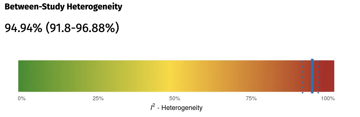
The section also provides summary information on the number of included studies/effect sizes, and their sample sizes. On the right side, a graph of the estimated between-study heterogeneity is displayed. Heterogeneity is quantified using the I2 value. Please note that, while I2 is commonly used in meta-analyses, it is not an absolute measure of heterogeneity (Borenstein et al., 2017), and its value depends on the size of the included studies.
Additionally, it is therefore also important to inspect the 95% prediction intervals, which are provided on the left side. These prediction intervals show the range of effect sizes to be expected in future studies, given the current evidence. These prediction intervals are a direct reflection of the between-study heterogeneity variance τ2, but are much easier to interpret than the latter (Inthout et al., 2016). If the 95% prediction interval does not contain zero, we can be quite confident that the effect of the treatment is robust across the various settings and contexts included in our meta-analysis.
Plots
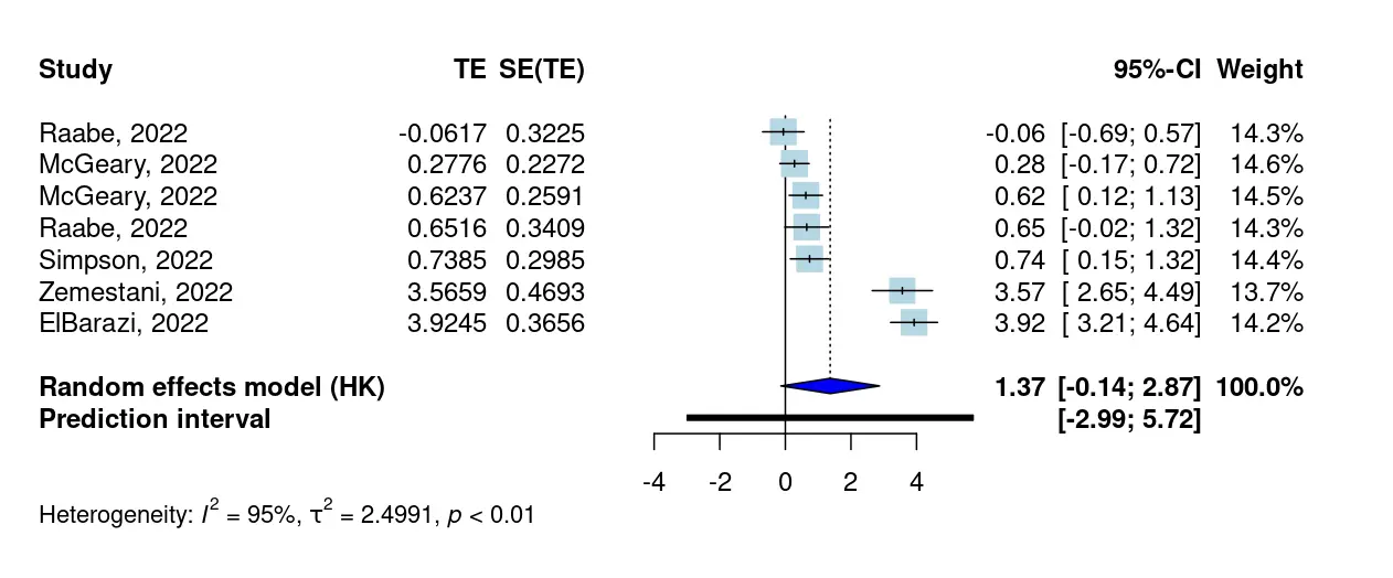
By default, two plots are generated to provide a summary of the results: a forest plot, and a drapery plot. All forest plots are sorted by effect size, which can help spot specific studies with very extreme effects. The plot provides the effect size for each study, as well as the weight assigned to it. At the bottom, the summary effect size is displayed along with the prediction interval.
Drapery plots (Rücker & Schwarzer, 2020) are a less commonly used but highly helpful method to visualize a pooled effect. These plots show how the prediction and confidence intervals change for different significance thresholds. The shaded blue area in the plot displays the prediction region for a future study, while the solid blue line gives the P-value function of the pooled effect (see e.g. Amrhein & Greenland, 2022).
Outliers
The “outliers” section displays a recalculated pooled effect when potential outliers are removed. This can be seen as a sensitivity analysis when studies with very extreme effects are excluded. Typically, removing outliers will lead to a pooled effect estimate that is less heterogeneous.
Outliers are identified as studies for which the 95% confidence interval lies outside the confidence interval of the pooled effect (Harrer et al., 2021, chap. 5.4.1). This “brute force” algorithm is easy to compute and therefore used within the application to enhance the speed. However, more sophisticated outlier and influence diagnostics may typically be preferred, and these analyses can be conducted with the metapsyTools package (see influence model).
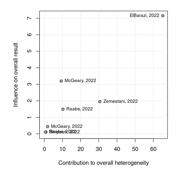
The right side of the section displays a Baujat plot, which visualizes studies' overall heterogeneity contribution against their influence on the overall result. This plot is based on a full influence analysis based on the “leave-one-out method” (Viechtbauer & Cheung, 2010). Studies in the right and top-right corners may be potential outliers or influential cases. Using the “exclude studies” filter in the study selection pane, it is possible to run a meta-analysis in which these studies are excluded specifically.
Publication Bias
The publication bias section displays the results of two methods: Egger’s (1997) regression test and P-curve (Simonsohn, Nelson & Simmons, 2014).
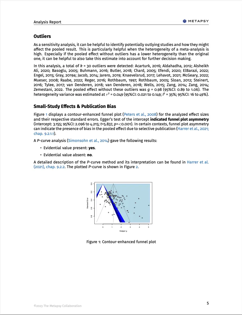
Egger’s regression test is shown on the left side. This method tests for asymmetry of the funnel plot, which is displayed on top. The funnel plot has been contour-enhanced by providing shaded blue areas for different significance regions: if statistical significance (i.e., P values below 0.05) serves as a selection mechanism concerning which studies are published, we would expect an excess of effects in the regions shaded in dark blue, but fewer studies in the white part of the plot, in which effects are not significant. Overall, a “lop-sided” (asymmetric) distribution of effects along the funnel indicates small-study effects (i.e., an excess of small studies with high effects) that can be indicative of publication bias (but does not have to).
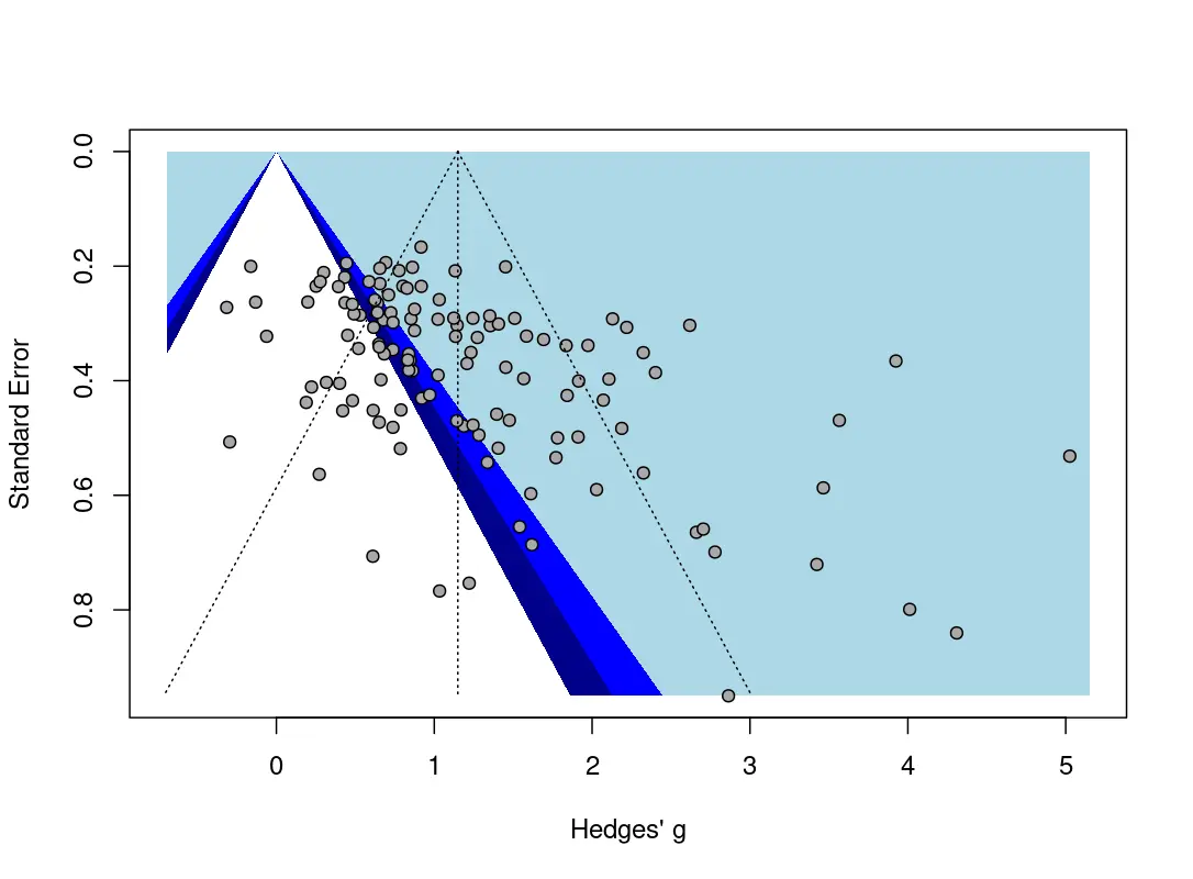
If Egger’s test of the intercept is significant, the funnel plot displays substantial asymmetry, and effects might be exaggerated due to publication bias. It is important to note that the power of this test depends heavily on the number of included studies. When there are few studies (say, below 10), a non-significant result should be interpreted cautiously. Overall, a non-significant finding of Egger’s test does not automatically indicate that no publication bias is present.
The right side of the section shows a P-curve. If there is a true effect and no selective publication, we would expect this curve to be right-skewed, with many highly significant findings, and fewer P values in the [0.3, 0.5) range. The P-curve method employs tests of flatness and right-skewness, which can be used to gauge if evidential evidence is present or absent. Please note that these two indicators are independent: it is also possible for P-curve to indicate that evidential evidence is neither present nor absent (for example because the analysis does not have sufficient power). More guidance on this method is provided in Harrer et al., 2021, chapter 9.2.2.
Risk of Bias
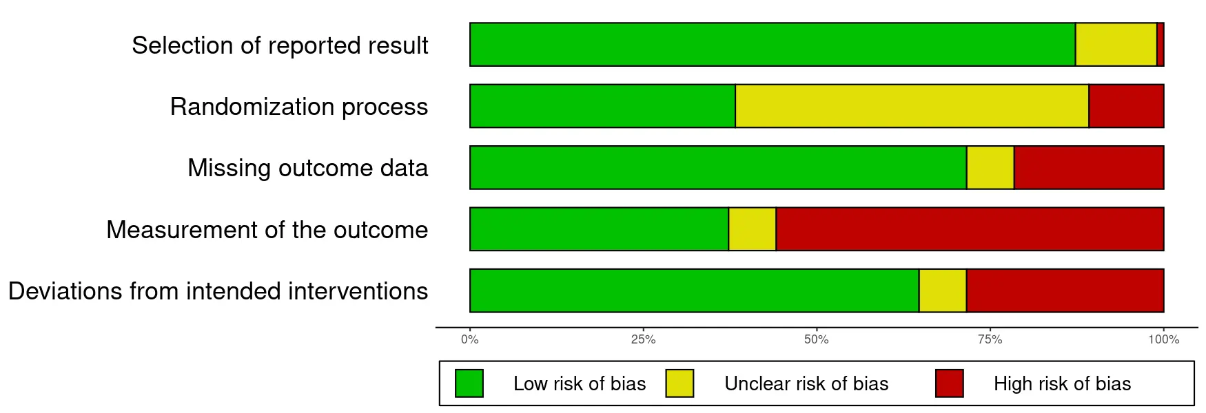
This section displays a summary plot of the risk of bias judgments for all included studies. It also gives the number and percentage of studies with an overall low risk of bias, and high risk of bias. Please note that the type of risk of bias rating applied in each database varies, as does the version of the RoB tool (version 1 or 2). Further details are provided in the documentation entry of each database.
Moderator Analysis
This section gives the results of moderator and subgroup analyses conducted as part of the meta-analysis. The “meta-regression” table displays the results of continuous moderators (e.g., publication year), while the “subgroup analysis” table is reserved for categorical moderators. In each table, P values are given on the right for the overall test of moderation. For the subgroup analyses, an additional P value is provided for the subgroup-specific effect estimate. Significant effects are shaded in light green. The “k” column shows the number of effect sizes in each subgroup, and teal-colored bars indicate the size of each subgroup. The “g” column shows the subgroup-conditional effect estimate, expressed as Hedges' g. Here, blue bars indicate the size of the pooled effect. The size of this bar is determined with reference to all estimates within the table.
By default, meta-regressions and subgroup analyses are presented for all variables included in the “Analyzed Moderators” field on top of the pane. Additional variables can be added by adjusting the selector, and then clicking on Re-run Meta-Analysis.
Analysis Settings
In this section on top of the results pane, it is possible to change the settings of the analysis. First, it is possible to change the estimator of the between-study heterogeneity variance τ2. Many different estimators are available, and which of them shows the best performance in specific settings is an ongoing research question (Langan et al., 2019).
In most applications, the restricted maximum likelihood (REML) estimator is used by default. This is also the default estimator used in common meta-analysis packages, such as metafor or meta. For some applications, this default setting is changed to another estimator (e.g., the Paule-Mandel estimator) to reflect the specific type of data included in a database. It is also possible to run a common/fixed-effect model instead, in which τ2 is fixed to zero.
By default, the Knapp-Hartung adjustment is applied for random-effects meta-analyses (see e.g. Hartung & Knapp, 2001). This correction does not apply to common/fixed-effect models. There can be rare cases when this correction leads to anticonservative results (Jackson et al., 2017), so it can be helpful to re-run the model without the correction to check for this. To do this, one has to uncheck the “Use Knapp-Hartung-Adjustments” checkbox, and then click on Re-run Meta-Analysis. The re-run button also has to be clicked first when another τ2 is to be used.
Report Generator
Most applications provide a reproducible report generator. The generator can be started by clicking on the Create Report button. The current state of the application is then compiled as a $\LaTeX$ file, and a PDF is downloaded.
Each generated report is provided with a distinct tracking ID, and the data used for the analyses is attached to it. All utilized filters are documented, enabling others to verify and reproduce the analyses. The appendix of the report shows the references from all the used studies, along with a detailed overview of the R and package versions employed for the meta-analysis.

Effect Explorer
A special meta-analysis application is the Metapsy effect explorer. This application has been developed for a broader audience and therefore provides less technical details than the “standard” online meta-analysis tools. The effect explorer allows to examine the pooled response rates and relative “risk” of response of psychotherapies for eight mental disorders (Depression, Borderline Personality Disorder, Generalized Anxiety Disorder, Obsessive Compulsive Disorder, Panic Disorder, Post-Traumatic Stress Disorder, Social Anxiety Disorder, Specific Phobia).
Like the other meta-analysis tools, this application also allows to generate a reproducible report of the results. This report also provides a more detailed technical description of the results and applied methodology. The underlying “meta-dataset” has been versioned and released with Zenodo.
Technical Stack
The online meta-analysis tools are hosted on the Linux server maintained by the Metapsy project (metapsy.dev). This server runs on Ubuntu 22.04 x64. It uses an installation of R (version 4.2.2), Python (version 3.10.12), shiny-server (Posit, 2023) and TeX Live.